Analyze activity data
SweatStack stores normalized timeseries, so an analysis script can query weeks or months of activity in a single call, without building an ingestion pipeline first. This guide covers two patterns: a one-off Python script for ad-hoc exploration, and a longitudinal query for trend analysis across many activities.
What you'll build
- A standalone Python script that fetches longitudinal cycling data and computes power and torque profiles
- An understanding of when to use a per-activity query and when to use a longitudinal query
Setup
The script uses uv, so it declares its dependencies inline. No requirements.txt, no virtualenv to manage.
Create analysis.py with this header:
# /// script
# requires-python = ">=3.10"
# dependencies = [
#     "sweatstack[pandas]",
#     "numpy",
#     "matplotlib",
# ]
# ///

from datetime import date, timedelta

import numpy as np
import pandas as pd
import matplotlib.pyplot as plt
from sweatstack import Client

client = Client()

client.authenticate()
sweatstack.authenticate() opens the browser once to sign in. The SDK caches the credentials for later runs.
Run the script with uv run analysis.py. The first run installs the dependencies. Later runs are fast.
Longitudinal queries: many activities at once
For trends across many activities, a longitudinal query returns a single timeseries DataFrame spanning the requested window:
data = client.activities.longitudinal.data(
    sport=["cycling.road"],
    start=date.today() - timedelta(days=90),
    metrics=["power", "cadence"],
)

print(f"{data['activity_id'].nunique()} activities, {len(data)} samples")
The timestamp column is timezone-aware UTC, so standard pandas resampling works once you make it the index:
weekly_max_power = data.set_index("timestamp")["power"].resample("W").max()
That resamples on UTC week boundaries. To group by the athlete's local calendar (day, week), use the naive local timestamp_local column instead. See Timezones.
The default metrics are duration, power, heart_rate, and speed. Pass metrics=[...] to request any other metric from the data model.
Activity metadata: per-activity summary data
When you don't need the timeseries, only the per-activity summary (sport, distance, duration, start time), use activities.list():
activities = client.activities.list(
    sport=["cycling.road"],
    start=date.today() - timedelta(days=90),
    output="pandas",
)
The API returns JSON, and with output="pandas" the SDK turns it into a DataFrame. Smaller payloads, faster queries. Use this when your analysis is at the activity level, not at the sample level.
Putting longitudinal queries to work: power and torque profiles
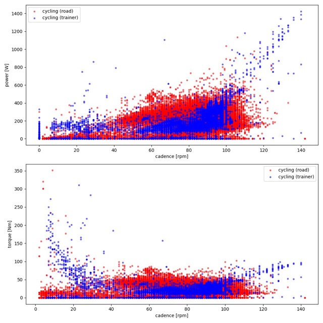
A worked example with a longitudinal query: compare the power-cadence relationship of road and trainer cycling.
# ... setup and client.authenticate() above ...

road = client.activities.longitudinal.data(
    sport=["cycling.road"],
    start=date.today() - timedelta(days=90),
    metrics=["power", "cadence"],
)

trainer = client.activities.longitudinal.data(
    sport=["cycling+stationary"],
    start=date.today() - timedelta(days=90),
    metrics=["power", "cadence"],
)

def torque(power, cadence):
    angular_velocity = cadence * (2 * np.pi / 60)
    t = pd.Series(index=power.index, dtype="float64")
    mask = angular_velocity > 0
    t[mask] = power[mask] / angular_velocity[mask]
    return t

road["torque"] = torque(road["power"], road["cadence"])
trainer["torque"] = torque(trainer["power"], trainer["cadence"])

fig, (ax_power, ax_torque) = plt.subplots(2, 1, figsize=(10, 10))

for df, color, label in [
    (road, "red", "Road"),
    (trainer, "blue", "Trainer"),
]:
    ax_power.scatter(df["cadence"], df["power"], color=color, marker=".", alpha=0.5, label=label)
    ax_torque.scatter(df["cadence"], df["torque"], color=color, marker=".", alpha=0.5, label=label)

ax_power.set(xlabel="cadence [rpm]", ylabel="power [W]")
ax_torque.set(xlabel="cadence [rpm]", ylabel="torque [Nm]")
ax_power.legend()
ax_torque.legend()

plt.show()
Tip: cache during iteration
While you iterate on the analysis itself, calling the API on every run is wasteful. Enable the SDK's local cache, and fix the start and end dates so the cache keys stay the same across runs:
import sweatstack
from sweatstack import Client

client = Client()

sweatstack.enable_cache()  # (1)!

data = client.activities.longitudinal.data(
    sport=["cycling.road"],
    start=date(2026, 1, 1),
    end=date(2026, 4, 1),  # fixed dates: the cache key stays the same
    metrics=["power", "cadence"],
)
- Caches longitudinal responses on disk, in the platform's cache directory. Pass
path="..."for a different directory.sweatstack.clear_cache()empties it.
Avoid date.today() while caching. The window shifts each day, and every run adds a new cache entry.
Next steps
- The data model covers every metric you can query, and how activities relate to traces, tests, and dailies.
- For analysis in an app (a web UI, deployed somewhere), see the Streamlit app and FastAPI app guides.
- For analysis of lab data (lactate tests, VO2max), see Tests and Metabolic profile.